



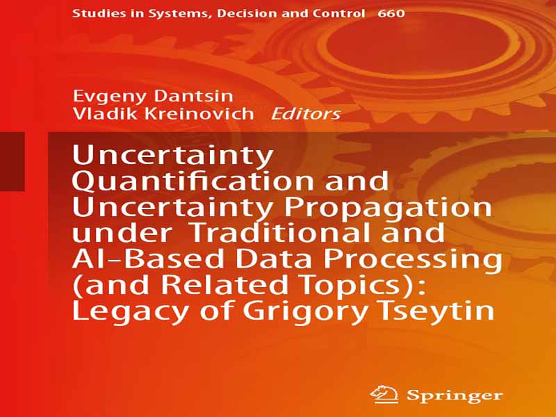
- عنوان کتاب: Uncertainty Quantification and Uncertainty Propagation under Traditional and AI-Based Data Processing
- نویسنده: Evgeny Dantsin, Vladik Kreinovich
- حوزه: عدم قطعیت
- سال انتشار: 2026
- تعداد صفحه: 335
- زبان اصلی: انگلیسی
- نوع فایل: pdf
- حجم فایل: 3.83 مگابایت
نیاز به پردازش دادهها اهداف اصلی علوم و مهندسی چیست؟ ما میخواهیم وضعیت فعلی جهان را بدانیم، میخواهیم وضعیت آینده جهان را پیشبینی کنیم و میخواهیم ابزارها را طراحی کنیم و اقداماتی انجام دهیم که این وضعیت آینده را تا حد امکان برای ما مفید کند. دانستن وضعیت به معنای دانستن مقادیر تمام کمیتهای فیزیکی توصیفکننده این وضعیت است. طراحی یک اقدام به معنای ارائه مقادیر مناسب برای کنترلهای مربوطه است. برخی از مقادیر فعلی کمیتهای فیزیکی را میتوانیم مستقیماً اندازهگیری کنیم، اما برای بسیاری از کمیتهای دیگر y، باید مقادیر آنها را بر اساس مقادیر کمیتهای مرتبط که اندازهگیری آنها آسانتر است x1، …، xn محاسبه کنیم. به عنوان مثال، ما نمیتوانیم مستقیماً فاصله تا یک ستاره دور یا مقدار نفت در یک میدان نفتی را اندازهگیری کنیم. و البته، نمیتوانیم مقادیر آینده کمیتهای فیزیکی یا پارامترهای کنترل بهینه را مستقیماً اندازهگیری کنیم: آنها باید بر اساس اطلاعات موجود، یعنی بر اساس مقادیر کمیتهای اندازهگیری شده x1، … محاسبه شوند. ، xn.. این محاسبه یک مورد خاص مهم از پردازش دادهها است. پردازش دادههای سنتی و مبتنی بر هوش مصنوعی به طور سنتی، الگوریتمهای پردازش دادهها عمدتاً از شناخت مدل فیزیکی موقعیت مربوطه، مدلی که در نهایت از تجزیه و تحلیل نتایج اندازهگیری قبلی حاصل میشود، ناشی میشوند. با این حال، اخیراً، بسیاری از پردازش دادهها توسط الگوریتمهای یادگیری ماشین (AI) انجام میشود، زمانی که یک برنامه به طور خودکار الگوریتمهای پردازش دادههای مورد نظر را از نتایج اندازهگیری شناخته شده تولید میکند، بدون اینکه نیازی به طراحی مدلهای ریاضی توسط محققان باشد. پردازش دادهها از دیدگاه ریاضی در همه این موارد، کمیت حاصل y به طور منحصر به فرد توسط مقادیر x1، …، xn. تعیین میشود، یعنی به زبان ریاضی، ما یک تابع y = f (x1، …، xn) داریم. ما فقط یک تابع به معنای ریاضی نداریم، بلکه یک تابع t داریم که میتواند محاسبه شود. چنین توابعی به عنوان قابل محاسبه یا سازنده شناخته میشوند. کمیسازی عدم قطعیت: مسائل رو به جلو و معکوس اندازهگیریها هرگز کاملاً دقیق نیستند. نتایج اندازهگیری xi. به طور کلی، تا حدودی با مقادیر واقعی (نامشخص) xi⁻ … مسئله کمیسازی عدم قطعیت معکوس از دیدگاه ریاضی در ریاضیات، موقعیتهایی که برای هر ε > 0. مقداری δ > 0. وجود دارد که برای آن، اگر xi را با دقت y δ. بدانیم، میتوانیم y = f (x1, . . . , xn) را با دقت y ε. تعیین کنیم، به خوبی شناخته شدهاند – توابع مربوطه پیوسته نامیده میشوند. ما علاقهمندیم که بتوانیم δ. را بر اساس ε. محاسبه کنیم. توابعی که چنین محاسبهای برای آنها امکانپذیر است، به عنوان توابع پیوسته محاسبهپذیر (یا سازنده) شناخته میشوند. نتیجه اساسی توسط گریگوری تسیتین یک نتیجه اساسی در این راستا در اواخر دهه 1950 – اوایل دهه 1960 توسط گریگوری تسیتین (1936-2022) اثبات شد. او ثابت کرد که هر تابع سازنده، از نظر سازنده پیوسته است، یعنی یک الگوریتم کلی وجود دارد که با داشتن یک تابع سازنده f(x1, …, xn) و مقدار مطلوب ε > 0، δ مربوطه را محاسبه میکند. از دیدگاه صرفاً ریاضی، ما یک الگوریتم کلی داریم که مسئله کمیسازی عدم قطعیت معکوس را حل میکند. اما آیا این تمام چیزی است که نیاز داریم؟ ما یک الگوریتم کلی داریم، اما آیا این الگوریتم عملی است؟ کاملاً مشخص است که بسیاری از الگوریتمها عملی نیستند، زیرا حتی در رایانههای مدرن، برای عملی بودن به زمان محاسبه بسیار زیادی نیاز دارند – گاهی اوقات زمان محاسبه بیشتر از طول عمر جهان. اوضاع در اوایل دهه 1960، زمانی که رایانهها بسیار کندتر بودند، حتی پیچیدهتر بود. بنابراین، برای عملیتر کردن الگوریتمهای خود – و دیگران -، تسیتین شروع به درگیر شدن در برنامهنویسی واقعی، از توسعه الگوریتمها گرفته تا توسعه کامپایلرهای کارآمد، کرد. او همچنین متوجه شد که بخش زیادی از دانش نه بر اساس فرمولها و مدلهای ریاضی، بلکه بر اساس کلمات زبان طبیعی وجود دارد: به عنوان مثال، بیشتر دانش پزشکی در زمان او اینگونه توصیف میشد. بنابراین، او به طور جدی شروع به تفکر در مورد زبانشناسی، حوزه تحقیقاتی که با متون زبان طبیعی سروکار دارد، کرد. بنابراین، او به یکی از پیشگامان زبانشناسی ریاضی و محاسباتی تبدیل شد…
Need for Data Processing What are the main objectives of science and engineering? We want to know the current state of the world, we want to predict the future state of the world, and we want to design gadgets and perform actions that would make this future state as beneficial to us as possible. Knowing the state means knowing the values of all the physical quantities characterizing this state. Designing an action means coming up with appropriate values of the corresponding controls. Some current values of the physical quantities we can measure directly, but for many other quantities y, we need to compute their values based on the values of the related easier-to-measure quantities x1, . . . , xn.. For example, we cannot directly measure the distance to a faraway star or the amount of oil in an oilfield. And, of course, we cannot directly measure the future values of ph ysical quantities or optimal control parameters: they have to be computed based on the available information, i.e., based on the values of measured quantities x1, . . . , xn.. This computation is an important particular case o f data processing. Traditional and AI-Based Data Processing Traditionally, algorithms for data processing mostly came from knowing the physical model of the corresponding situation, the model that comes, eventually, from analyzing previous measurement results. However, lately, a lot of data processing is done by machine learning (AI) algorithms, when a program automatically produced the desired data processing algorithms from the known measurement results, without the need for researchers to design mathematical models. Data Processing from the Mathematical Viewpoint In all these cases, the resulting quantity y is uniquely determined by the values x1, . . . , xn., i.e., in mathematical terms, we have a function y = f (x1, . . . , xn).. We do not just have a function in the mathematical sense, we have a function t hat can be computed. Such functions are known as computable, or constructive. Uncertainty Quantification: Forward and Inverse Problems Measurements are never absolutely accurate. Measurement results xi . are, in general, somewhat differ ent from the actual (unknown) values xi . of the corresponding quantities. Because of this measurement uncertainty (also known as measurement error), the value y = f (x1, . . . , xn). that we get by processing measurement results xi . is, in general, different from the value y = f (x1, . . . , xn). that we would have got if we knew the exact values xi .. It is therefore important to quantify the resulting uncertainty in y, i.e., to know how uncertainty in the inputs xi . affects the accuracy with which we can compute y. This is a forward problem of uncertainty quantification. It is also important to solv e the corresponding inverse problem, when we know the accuracy ε > 0. with which we want to determine y, and we need to find out with what accuracy we need to measure xi . to maintain the desired accuracy in y. Inverse Uncertainty Quantification Problem from the Mathematical Viewpoint In mathematics, situations when for every ε > 0. there is a value δ > 0. for which, if we know xi . with accurac y δ., then we can determine y = f (x1, . . . , xn). with accurac y ε. are well known—the corresponding functions are called continuous. We are interested in being able to compute δ. based on ε.. Functions for which such computation is possible are kno wn as computably (or constructively) continuous. Fundamental Result by Grigory Tseytin A fundamental result in this direction was proven in the late 1950s—early 1960s by Grigory Tseytin (1936–2022). He proved that every constructive f unction is constructively continuous, i.e., that there is a general algorithm that, given a constructive function f (x1, . . . , xn). and the desired value ε > 0., computes the corresponding δ.. From the purely mathematical viewpoint, we have a general algorithm that solves the inverse uncertainty quantification problem. But Is This All We Need? We have a general algorithm, but is this algorithm practical? It is well known that many algorithms are not practical, since even on modern computers, they would require too much computation time to be practical— sometimes more computation time than the lifetime of the Universe. The situation was even more complicated in the early 1960s, when computers were much slower. So, to make his—and others’—algorithms more practical, Tseytin started to get involved in the actual programming, from developing algorithms to developing efficient compilers. He also realized that a lot of knowledge exists not in terms of the formulas and mathematical models, but rather in terms of words from natural language: this is, e.g., how most medical knowledge was described at his time. So, he started seriously thinking about linguistics, research area that deals with natural-language texts. Thus, he became one of the pioneers of mathematical and computational linguistics. Computing and linguistics eventually became Tseytin’s main research areas.
این کتاب را میتوانید از لینک زیر بصورت رایگان دانلود کنید:
Download: Uncertainty Quantification
















نظرات کاربران